Softmax Layer
The filter weights that were initialized with random numbers become task specific as we learn.
Learning is a process of changing the filter weights so that we can expect a particular output mapped for
each data samples.
Consider the task of handwritten digit recognition [LBD+90].
Here, we attempt to map images ( pixels) to an integer
 ![y \in [0,1 \dots 9]](../_images/math/3aa262b4955e429392f8c749edfba0daa6ecb917.png) .
MNIST is the perfect dataset for this example, which was desigend for this purpose.
MNIST images typically look as follows:
.
MNIST is the perfect dataset for this example, which was desigend for this purpose.
MNIST images typically look as follows:
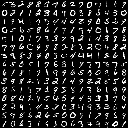
Fig. 6 MNIST dataset of handwritten character recognition.
Learning in a neural network is typically achieved using the back-prop learning strategy.
At the top end of the neural network with as many layers is a logistic regressor that feeds off of the last layer of activations,
be it from a fully-connected layer as is conventional or a convolutional layer such as in some recent network implementations
used in image segmentation [LSD15].
When the layer feeding into a softmax layer is a dot-product layer with an identity activation  , we refer to the inputs
often as logits.
In modern neural networks, the logits are not limited in operation with any activations.
Often, this regressor is also implemented using a dot-product layer, for logistic regression is simply
a dot-product layer with a softmax activation.
, we refer to the inputs
often as logits.
In modern neural networks, the logits are not limited in operation with any activations.
Often, this regressor is also implemented using a dot-product layer, for logistic regression is simply
a dot-product layer with a softmax activation.
A typical softmax layer is capable of producing the probability distribution over the labels ![y \in [0, 1, \dots c]](../_images/math/c8c83ce3d27f2d7d7c4e1b227ec5648f3a83d81c.png) that we want to predict.
Given an input image
that we want to predict.
Given an input image  ,
,  is estimated as follows,
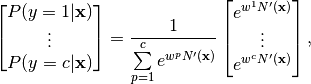
where,  is the weight matrix of the dot-product layer preceding the softmax layer
with
is the weight matrix of the dot-product layer preceding the softmax layer
with  representing the weight vector that produces the output of the class
  and
and
 is the output of the layer in the network
  , immediately preceding
this dot-product-softmax layer.
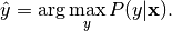
The label that the network predicts
, immediately preceding
this dot-product-softmax layer.
The label that the network predicts  , is the maximum of these probabilities,
Implementation
I implemented the softmax layer as follows:
- Use a
lenet.layers.dot_product_layer()with 10 neurons andidentityactivation.- Use a
lenet.layers.softmax_layer()to produce the softmax.
In the softmax layer, we can return computational graph nodes to predictions, logits and softmax. The reason for using logits will become clear in the next section when we discuss errors and back prop. Essentially, we will create a layer that will look like the following image in its tensorboard visualization:
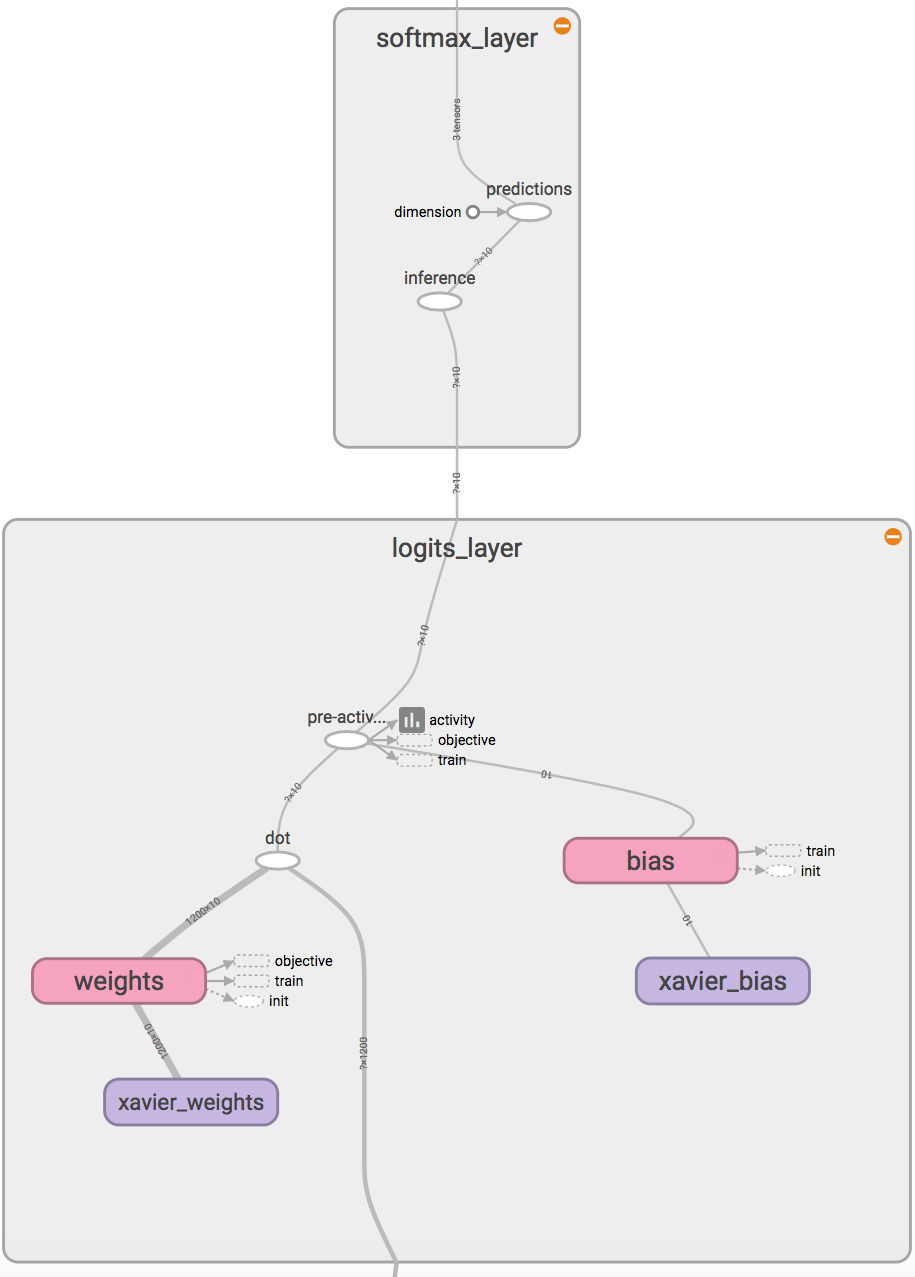
Fig. 7 Softmax Layer implementation.
The logits layer is a lenet.layers.dot_product_layer() with identity activation (no activation).
The inference node will produce the softmax and the prediction node will produce the label predicted.
Th softmax layer is implemented as:
inference = tf.nn.softmax(input, name = 'inference')
predictions = tf.argmax(inference, 1, name = 'predictions')
Where tf.nn.softmax() and tf.nn.argmax() have similar syntax as the theano counterparts.
To have the entire layer, in the lenet.network.lenet5 which is where these layer methods are called,
I use the following strategy:
# logits layer returns logits node and params = [weights, bias]
logits, params = lenet.layers.dot_product_layer  (
                                        input = fc2_out_dropout,
                                        neurons = C,
                                        activation = 'identity',
                                        name = 'logits_layer')
# Softmax layer returns inference and predictions
inference, predictions = lenet.layers.softmax_layer (
                                        input = logits,
                                        name = 'softmax_layer' )
Where C is a globally defined variable with C=10 defined in lenet.gloabl_definitions file.
The layer definitions can be seen in full in the documentation of the lenet.layers.softmax_layer() method.