Dot-Product Layers
Consider a  vector of inputs
 ![\mathbf{x} \in [x_0,x_1, \dots x_d]](../_images/math/f846981ea55a04b71210fda88c64f9337946c0d5.png) of
of  dimensions.
This may be a vectorized version of the image or may be the output of a preceding layer.
Consider a dot-product layer containing
dimensions.
This may be a vectorized version of the image or may be the output of a preceding layer.
Consider a dot-product layer containing  neurons.
The
neurons.
The  th neuron in this layer will simply perform the following operation,
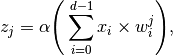
where,  is typically an element-wise monotonically-increasing function that scales the output of the dot-product.
is commonly referred to as the activation function.
The activation function is used typically as a threshold, that either turns ON (or has a level going out) or OFF, the neuron.
The neuron output that has been processed by an activation layer is also referred to as an activity.
Inputs can be processed in batches or mini-batches through the layer.
In these cases
is typically an element-wise monotonically-increasing function that scales the output of the dot-product.
is commonly referred to as the activation function.
The activation function is used typically as a threshold, that either turns ON (or has a level going out) or OFF, the neuron.
The neuron output that has been processed by an activation layer is also referred to as an activity.
Inputs can be processed in batches or mini-batches through the layer.
In these cases  is a matrix in
  , where
  is the batch size.
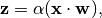
Together, the vectorized output of the layer is the dot-product operation between the weight-matrix of the layer and the input signal batch,
is the batch size.
Together, the vectorized output of the layer is the dot-product operation between the weight-matrix of the layer and the input signal batch,
where,  ,
,  and the
  element of
 represents the output of the
  neuron for the
  sample of input.
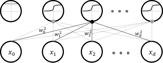
Fig. 1 A typical dot-product layer
The above figure shows such a connectivity of a typical dot-product layer.
This layer takes in an input of dimensions and produces an output of dimensions.
From the figure, it should be clear as to why dot-product layers are also referred to as fully-connected layers.
These weights are typically learnt using back-propagation and gradient descent [RHW85].
Implementation
Dot-product layers are implemented in tensorflow by using the tf.matmul() operation, which is a
dot product operation. Consider the following piece of code:
# Open a new scope
with tf.variable_scope('fc_layer') as scope:
    # Initialize new weights
    weights = tf.Variable(initializer([input.shape[1].value,neurons], name = 'xavier_weights'),\
                                        name = 'weights')
    # Initialize new bias
    bias = tf.Variable(initializer([neurons], name = 'xavier_bias'), name = 'bias')
    # Perform the dot product operation
    dot = tf.nn.bias_add(tf.matmul(input, weights, name = 'dot'), bias, name = 'pre-activation')
    activity = tf.nn.relu(dot, name = 'activity' )  # relu is our alpha and activity is z

    # Add things to summary
    tf.summary.histogram('weights', weights)
    tf.summary.histogram('bias', bias)
    tf.summary.histogram('activity', activity)
This code block is very similar to how a dot product would be implemented in theano. For instance, in yann I implemented a dot product layer like so:
w_values = numpy.asarray(0.01 * rng.standard_normal(
            size=(input_shape[1], num_neurons)), dtype=theano.config.floatX)
weights = theano.shared(value=w_values, name='weights')
b_values = numpy.zeros((num_neurons,), dtype=theano.config.floatX)
bias = theano.shared(value=b_values, name='bias')
dot = T.dot(input, w) + b
activity = theano.nnet.relu(dot)
We can already see that the theano.shared() equivalent in tensorflow is the tf.Variable(). They
work in similar fashion as well. tf.Variable() is a node in a computational graph, just like theano.shared()
variable. Operationally, the rest is easy to infer from the code itself.
There are some newer elements in the tensorflow code. Tensorflow graph components (variables and ops)
could be enclosed using tf.variable_scope() declarations. I like to think of them as boxes to put things in
literally. Once we go through tensorboard, it can be noticed that sometimes they literally are boxes.
For instance, the following is a tensorboard visualization of this scope.
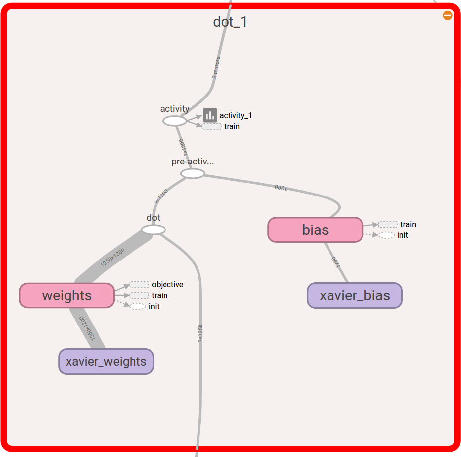
Fig. 2 A dot-product layer scope visualized in tensorboard
The initialization is also nearly the same.
The API for the Xavier initializer can be found in the lenet.support.initializer() module.
Tensorflow summaries is an entirely new option
that is not available clearly in theano. Summaries are hooks that can write down or export information
presently stored in graph components that can be used later by tensorboard to read and present in a nice
informative manner. They can be pretty much anything of a few popular hooks that tensorflow allows.
the summary.histogram allows us to track the histogram of particular variables as they change
during iterations. We will go into more detail about summaries as we study the lenet.trainer.trainer.summaries() method, but
at this moment you can think of them as hooks that export data.
The entire layer class description can be found in the lenet.layers.dot_product_layer() method.