Additional Notes¶

Thanks for checking out my tutorial, I hope it was useful.

Stochastic Gradient Descent¶

Since in theano we use the theano.tensor.grad() to estimate gradients from errors and back propagate ourselves, it was easier to understand and learn about various minimization algorithms. In yann for instance, I had to write all the optimizers I used, by hand as seen here. In tensorflow everything is already provided to us in the Optimizer module. I could have written out all the operations myself, but I copped out by using the in-built module. Therefore, here is some notes on how to minimize an error.

Consider the prediction $\hat{y}$ . Consider we come up with some error $e$ , that measure how different is $\hat{y}$ with $y$ . In our tutorial, we used the categorical cross-entropy error. If $e$ were a measure of error in this prediction, in order to learn any weight $w$ in the network, we can acquire its gradient $\frac{\partial e}{\partial w}$ , for every weight $w$ in the network using the chain rule of differentiation. Once we have this error gradient, we can iteratively learn the weights using the following gradient descent update rule:

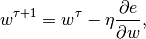
$w^{\tau+1} = w^{\tau} - \eta \frac{\partial e}{\partial w},$

where, $\eta$ is some predefined rate of learning and $\tau$ is the iteration number. It can be clearly noticed in the back-prop strategy outlined above that the features of a CNN are learnt with only one objective - to minimize the prediction error. It is therefore to be expected that the features learnt thusly, are specific only to those particular tasks. Paradoxically, in deep CNNs trained using large datasets, this is often not the typical observation.

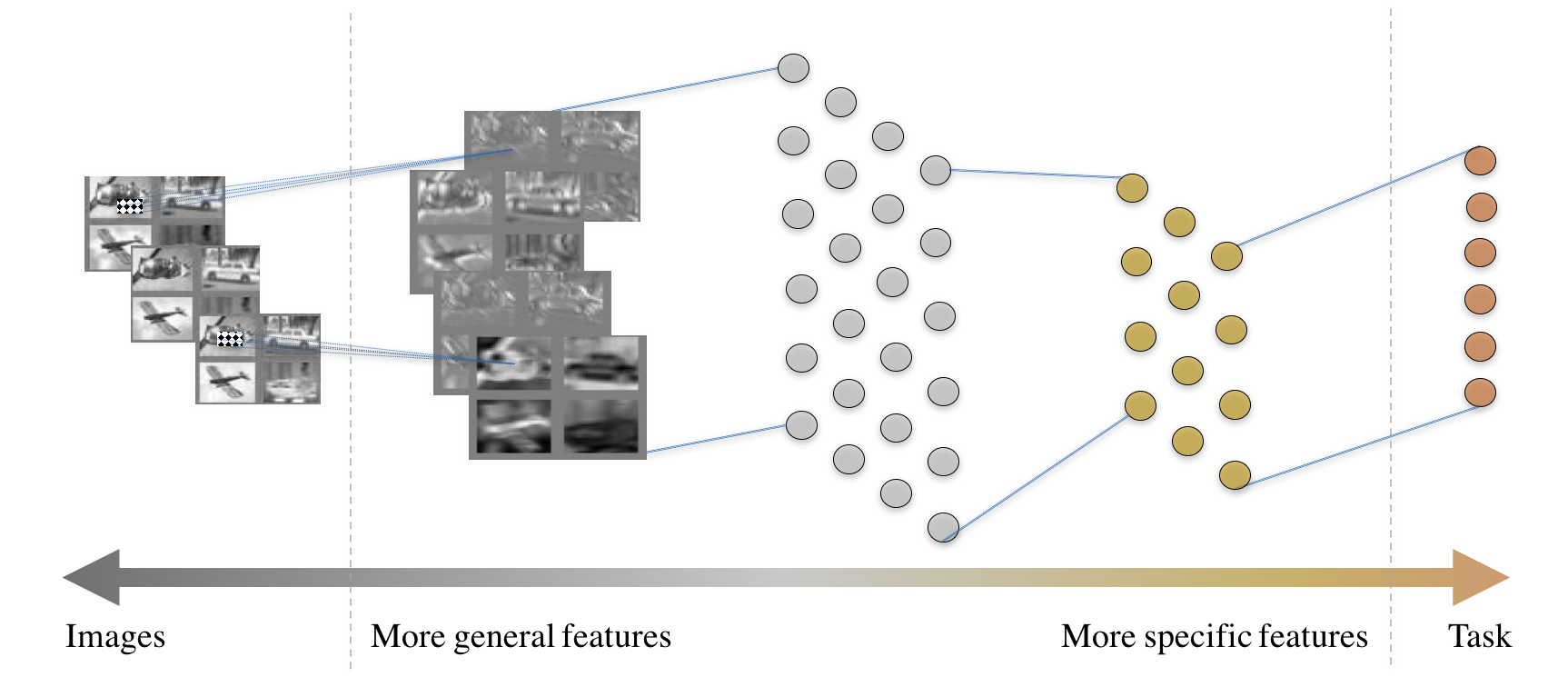
Fig. 12 The anatomy of a typical convolutional neural network.

In most CNNs, we observe as illustrated in the figure above, that the anatomy of the CNN and the ambition of each layer is contrived meticulously. The features that are close to the image layer are more general (such as edge detectors or Gabor filters) and those that are closer to the task layer are more task-specific.

Off-the-shelf Downloadable networks¶

Given this observation among most popular CNNs, modern day computer vision engineers prefer to simply download off-the-shelf neural networks and fine-tune it for their task. This process involves the following steps. Consider that a stable network $N$ is well-trained on some task $T$ that has a large dataset and compute available at site. Consider that the target for an engineer is build a network $n$ that can make inferences on task $t$ . Also assume that these two tasks are somehow related, perhaps $T$ was visual object categorization on ImageNet and $t$ on the COCO dataset [LMB+14] or the Caltech-101/256 datasets [FFFP06]. To learn the task on $t$ , one could simply download $N$ , randomly reinitialize the last few layers (at the extreme case reinitialize only the softmax layer) and continue back-prop of the network to learn the task $t$ with a smaller eta. It is expected that $N$ is very well-trained already that they could serve as good initialization to begin fine-tuning the network for this new task. In some cases where enough compute is not available to update all the weights, we may simply choose to update only a few of the layers close to the task and leave the others as-is. The first few layers that are not updated are now treated as feature extractors much the same way as HOG or SIFT.

Some networks capitalized on this idea and created off-the-shelf downloadable networks that are designed specifically to work as feed-forward deterministic feature extractors. Popular off-the-shelf networks were the decaf [DJV+14] and the overfeat [SEZ+13]. Overfeat in particular was used for a wide-variety of tasks from pulmonary nodule detection in CT scans [vGSJC15] to detecting people in crowded scenes [SAN16]. While this has been shown to work to some degrees and has been used in practice constantly, it is not a perfect solution and some problems have known to exist. This problem is particularly striking when using a network trained on visual object categorization and fine-tuned for tasks in medical image.

Distillation from downloaded networks¶

Another concern with this philosophy of using off-the-shelf network as feature extractors is that the network $n$ is also expected to be of the same size as $N$ . In some cases, we might desire a network of a different architecture. One strategy to learn a different network using a pre-trained network is by using the idea of distillation [HVD15], [BRMW15]. The idea of distillation works around the use of a temperature-raised softmax, defined as follows:

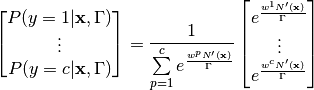
$\begin{bmatrix} P(y = 1 \vert \mathbf{x},\Gamma) \\ \vdots \\ P(y = c \vert \mathbf{x},\Gamma) \end{bmatrix} = \frac{1}{\sum\limits_{p=1}^c e^\frac{{w^{p}N'(\mathbf{x})}}{\Gamma}} \begin{bmatrix} e^\frac{w^{1}N'(\mathbf{x})}{\Gamma} \\ \vdots \\ e^\frac{w^{c}N'(\mathbf{x})}{\Gamma} \end{bmatrix}$

This temperature-raised softmax for $\Gamma>1$ ( $\Gamma=1$ is simply the original softmax) provides a softer target which is smoother across the labels. It reduces the probability of the most probable label and provides rewards for the second and third most probable labels also, by equalizing the distribution. Using this dark-knowledge to create the errors $e$ (in addition to the error over predictions as discussed above), knowledge can be transferred from $N$ , during the training of $n$ . This idea can be used to learn different types of networks. One can learn shallower [VL16] or deeper [RBK+14] networks through this kind of mentoring.